2  The Art and Science of Machine Learning

Learning lies at the heart of intelligence, whether natural or artificial. In this chapter, we will embark on a fascinating exploration of the fundamental principles that enable machines to learn from experience. Together, we will examine both the theoretical foundations that provide a rigorous mathematical basis for machine learning, as well as the practical considerations that shape the design and implementation of modern learning systems. Our journey will take us from the historical roots of the field through to the cutting-edge research defining the current state of the art and the open challenges guiding future directions. By the end of this chapter, you will have built a comprehensive understanding of how machines can acquire, represent, and apply knowledge to solve complex problems and enhance decision-making across a wide range of domains.

To make our exploration as engaging and accessible as possible, I will aim to break down complex ideas into more easily digestible parts, building up gradually to the more advanced concepts. Along the way, I will make use of intuitive analogies, illustrative examples, and step-by-step explanations to help illuminate key points. Please feel free to ask questions or share your own insights at any point - learning is an interactive process and your contributions will only enrich our discussion!

With that in mind, let’s begin our journey into the art and science of machine learning.

2.1 Origins and Evolution

To fully appreciate the current state and future potential of machine learning, it is helpful to understand its historical context and developmental trajectory. In this section, we will trace the origins of the field and highlight the pivotal advances that have shaped its evolution.

2.1.1 Historical Context

The dream of creating intelligent machines that can learn and adapt has captivated the human imagination for centuries. In mythology and folklore around the world, we find stories of animated beings imbued with ‘artificial’ intelligence, from the golems of Jewish legends to the mechanical servants of ancient China. These ageless visions speak to a deep fascination with the idea of breathing life and cognizance into inanimate matter.

However, the emergence of machine learning as a scientific discipline is a more recent development, tracing its origins to the mid-20th century. In a profound sense, the birth of machine learning as we know it today arose from the convergence of several key intellectual traditions:

Artificial intelligence - The quest to create machines capable of intelligent behavior

Statistics and probability theory - The mathematical tools for quantifying and reasoning about uncertainty

Optimization and control theory - The principles for automated decision-making and goal-directed behavior

Neuroscience and cognitive psychology - The scientific study of natural learning in biological systems

Each of these tributaries contributed essential ideas and techniques that merged together to form the foundations of modern machine learning.

Some key milestones in the early history of the field:

• 1943 - Warren McCulloch and Walter Pitts publish “A Logical Calculus of the Ideas Immanent in Nervous Activity”, laying the groundwork for artificial neural networks

• 1950 - Alan Turing proposes the “Turing Test” in his seminal paper “Computing Machinery and Intelligence”, providing an operational definition of machine intelligence

• 1952 - Arthur Samuel writes the first computer learning program, which learned to play checkers better than its creator

• 1957 - Frank Rosenblatt invents the Perceptron, an early prototype of artificial neural networks capable of learning to classify visual patterns

• 1967 - Covering numbers and the Vapnik–Chervonenkis dimension (VC dimension) introduced in the groundbreaking work of Vladimir Vapnik and Alexey Chervonenkis, providing the foundations for statistical learning theory

These pioneering efforts laid the conceptual and technical groundwork for the subsequent decades of research that grew the field into the thriving discipline it is today.

2.1.2 From Rule-Based to Learning Systems

In its early stages, artificial intelligence research focused heavily on symbolic logic and deductive reasoning. The prevailing paradigm was that of “expert systems” - computer programs that encoded human knowledge and expertise in the form of explicit logical rules. A canonical example was MYCIN, a program developed at Stanford University in the early 1970s to assist doctors in diagnosing and treating blood infections. MYCIN’s knowledge base contained hundreds of IF-THEN rules obtained by interviewing expert physicians, such as:

IF (organism-1 is gram-positive) AND 
   (morphology of organism-1 is coccus) AND
   (growth-conformation of organism-1 is chains)
THEN there is suggestive evidence (0.7) that
     the identity of organism-1 is streptococcus

By chaining together inferences based on these rules, MYCIN could arrive at diagnostic conclusions and treatment recommendations that rivaled those of human specialists in its domain.

However, the handcrafted knowledge-engineering approach of early expert systems soon ran into serious limitations:

• Knowledge acquisition bottleneck: Extracting and codifying expert knowledge proved to be extremely time-consuming and prone to inconsistencies and biases.

• Brittleness and inflexibility: Rule-based systems struggled to handle noisy data, adapt to novel situations, or keep up with changing knowledge.

• Opaque “black box” reasoning: The complex chains of inference generated by expert systems were often difficult for humans to inspect, understand, and debug.

• Inability to learn from experience: Once programmed, rule-based systems remained static and could not automatically improve their performance or acquire new knowledge.

These shortcomings highlighted the need for a fundamentally different approach - one that could overcome the rigidity and opacity of handcrafted symbolical rules and instead acquire knowledge directly from data.

2.1.3 The Statistical Revolution

The critical shift from rule-based to learning systems was catalyzed by two key insights: Many real-world domains are intrinsically uncertain and subject to noise, necessitating a probabilistic treatment. Expertise is often implicit and intuitive rather than explicit and axiomatic, making it more amenable to statistical extraction than symbolic codification.

Consider again the task of medical diagnosis that systems like MYCIN sought to automate. While it is possible to elicit a set of logical rules from a human expert, there are several complicating factors:

• Patients present with constellations of symptoms that are imperfectly correlated with underlying disorders.

• Diagnostic tests yield results with varying levels of accuracy and associated error rates.

• Diseases evolve over time, manifesting differently at different stages.

• Treatments have uncertain effects that depend on individual patient characteristics.

• New diseases emerge and existing ones change in their prevalence and manifestation over time. In such an environment, definitive logical rules are the exception rather than the norm. Instead, diagnosis is fundamentally a process of probabilistic reasoning under uncertainty, based on a combination of empirical observations and prior knowledge.

The key innovation that unlocked machine learning was to reframe the challenge in statistical terms:

• Instead of trying to manually encode deterministic rules, the goal became to automatically infer probabilistic relationships from observational data.

• Rather than requiring knowledge to be explicitly enumerated, learning algorithms aimed to implicitly extract latent patterns and regularities.

• In place of brittle logical chains, models learned robust statistical associations that could gracefully handle noise and uncertainty.

This shift in perspective opened up a powerful new toolbox of techniques at the intersection of probability theory and optimization. Some key formal developments:

• Maximum likelihood estimation (Ronald Fisher, 1920s): A principled framework for inferring the parameters of statistical models from observed data.

• The perceptron (Frank Rosenblatt, 1957): A simple type of artificial neural network capable of learning to classify linearly separable patterns.

• Stochastic gradient descent (Herbert Robbins & Sutton Monro, 1951): An efficient optimization procedure well-suited to large-scale machine learning problems.

• Backpropagation (multiple independent discoveries, 1970s-1980s): An algorithm for training multi-layer neural networks by propagating errors backwards through the network.

• The VC dimension (Vladimir Vapnik & Alexey Chervonenkis, 1960s-1970s): A measure of the capacity of a hypothesis space that quantifies the conditions for stable learning from finite data.

• Maximum margin classifiers and support vector machines (Vladimir Vapnik et al., 1990s): Powerful discriminative learning algorithms with strong theoretical guarantees.

Together, innovations like these provided the foundations for statistical learning systems that could effectively extract knowledge from raw data. They set the stage for the following decades of progress that would see machine learning mature into one of the most transformative technologies of our time.

2.2 Understanding Learning Systems

Having reviewed the historical context and key conceptual shifts behind the emergence of machine learning, we are now in a position to examine learning systems in greater depth. In this section, we will explore the fundamental principles that define the learning paradigm, the central role played by data, and the nature of the patterns that learning uncovers.

2.2.1 The Learning Paradigm

At its core, machine learning represents a radical departure from traditional programming approaches. To appreciate this, it is helpful to consider how we might go about solving a complex task such as object recognition using classical programming:

First, we would need to sit down and think hard about all the steps involved in identifying objects in images. We might come up with rules like:

• “an eye has a roughly circular shape”
• “a nose is usually located below the eyes and above the mouth”
• “a face is an arrangement of eyes, nose and mouth”, etc.

Next, we would translate these insights into specific programmatic instructions:

• “scan the image for circular regions”
• “check if there are two such regions in close horizontal proximity”
• “label these candidate eye regions”, etc.

We would then need to painstakingly debug and refine our program to handle all the edge cases and sources of variability we failed to consider initially.

If our program needs to recognize additional object categories, we would have to return to step 1 and repeat the whole arduous process for each new class.

The classical approach places the entire explanatory burden on the human programmer - we start from a blank slate and must explicitly spell out every minute decision and edge case handling routine.

In contrast, the machine learning approach follows a very different recipe:

First, we collect a large dataset of labeled examples (e.g. images paired with the names of the objects they contain). We select a general-purpose model family that we believe has the capacity to capture the relevant patterns (e.g. deep convolutional neural networks for visual recognition). We specify a measure of success (e.g. what fraction of the images are labeled correctly) - this is our objective function.

We feed the dataset to a learning algorithm that automatically adjusts the parameters of the model so as to optimize the objective function on the provided examples. We evaluate the trained model on a separate test set to assess its ability to generalize to new cases.

Notice how the emphasis has shifted:

• Rather than having to explain “how” to solve the task, we provide examples of “what” we want and let the learning algorithm figure out the “how” for us.

• Instead of handcrafting detailed solution steps, we select a flexible model and offload the burden of tuning its parameters to an optimization procedure.

• In place of open-ended debugging, we can run controlled experiments to objectively measure generalization to unseen data.

For a more concrete illustration, consider how we might apply machine learning to the task of spam email classification:

import numpy as np
from sklearn.model_selection import train_test_split
from sklearn.feature_extraction.text import CountVectorizer
from sklearn.naive_bayes import MultinomialNB
from sklearn.metrics import accuracy_score

# 1. Collect labeled data 
emails, labels = load_email_data()

# 2. Select a model family
vectorizer = CountVectorizer()  # convert email text to word counts
classifier = MultinomialNB()    # naive Bayes with multinomial likelihood

# 3. Specify an objective function
def objective(model, X, y):  
    return accuracy_score(y, model.predict(X))
    
# 4. Feed data to a learning algorithm
# learn a spam classifier from 70% of the data 
train_emails, test_emails, train_labels, test_labels = train_test_split(
        emails, labels, train_size=0.7, stratify=labels)  
X_train = vectorizer.fit_transform(train_emails)
classifier.fit(X_train, train_labels)

# 5. Evaluate generalization on held-out test set  
X_test = vectorizer.transform(test_emails)
print("Test accuracy:", objective(classifier, X_test, test_labels))

This simple example illustrates the key ingredients:

• Data: A collection of example emails, along with human-provided labels indicating whether each one is spam or not.

• Model: The naive Bayes classifier, which specifies the general form of the relationship between the input features (word counts) and output labels (spam or not spam) in terms of probabilistic assumptions.

• Objective: The accuracy metric, which quantifies the quality of predictions made by the model in terms of the fraction of emails that are labeled correctly.

• Learning algorithm: The fit method of the classifier, which takes in the training data and finds the model parameters that maximize the likelihood of the observed labels.

• Generalization: The trained model is evaluated not on the data it was trained on, but rather on a separate test set that was held out during training. This provides an unbiased estimate of how well the model generalizes to new, unseen examples.

Of course, this is just a toy example intended to illustrate the basic flow. Real-world applications involve much larger datasets, more complex models, and more challenging prediction tasks. But the fundamental paradigm remains the same: by optimizing an objective function on a sample of training data, learning algorithms can automatically extract useful patterns and knowledge that generalize to novel situations.

2.2.2 Learning from Data

As the spam classification example makes clear, data plays a first-class role in machine learning. Indeed, one of the defining characteristics of the field is its focus on automatically extracting knowledge from empirical observations, rather than relying solely on human-encoded expertise. In this section, we take a closer look at how learning systems leverage data to acquire and refine their knowledge.

To begin, it is useful to clarify what we mean by “data” in a machine learning context. At the most basic level, a dataset is a collection of examples, where each example (also known as a “sample” or “instance”) provides a concrete instantiation of the task or phenomenon we wish to learn about. In the spam classification scenario, for instance, each example corresponds to an actual email message, along with a label indicating whether it is spam or not.

More formally, we can think of an example as a pair (x,y), where:

• \(x\) is a vector of input features that provide a quantitative representation of the relevant properties of the example. In the case of emails, the features might be counts of various words appearing in the message.

• \(y\) is the target output variable that we would like to predict given the input features. For spam classification, \(y\) is a binary label, but in general it could be a continuous value (regression), a multi-class label (classification), or a more complex structure like a sequence or image.

A dataset, then, is a collection of n such examples:

\[D = {(x₁, y₁), ..., (xₙ, yₙ)}\]

The goal of learning is to use the dataset \(D\) to infer a function \(f\) that maps from inputs to outputs:

\(f: X → Y\) such that \(f(x) ≈ y\) for future examples \((x,y)\) that were not seen during training.

With this formalism in mind, we can identify several key properties of data that are crucial for effective learning:

• Representativeness: To generalize well, the examples in \(D\) should be representative of the distribution of inputs that will be encountered in the real world. If the training data is systematically biased or skewed relative to the actual test distribution, the learned model may fail to perform well on new cases.

• Quantity: In general, more data is better for learning, as it provides a richer sampling of the underlying phenomena and helps the model to avoid overfitting to accidental regularities. The amount of data needed to achieve a desired level of performance depends on the complexity of the task and the expressiveness of the model class.

• Quality: The utility of data for learning can be undermined by issues like noise, outliers, and missing values. Careful data preprocessing, cleaning, and augmentation are often necessary to ensure that the model is able to extract meaningful signal.

• Diversity: For learning to succeed, the training data must contain sufficient variability along the dimensions that are relevant for the task at hand. If all the examples are highly similar, the model may fail to capture the full range of behaviors needed for robust generalization.

• Labeling: In supervised learning tasks, the quality and consistency of the output labels is critical. Noisy, ambiguous, or inconsistent labels can severely degrade the quality of the learned model.

To make these ideas more concrete, let’s return to the spam classification example. Consider the following toy dataset:

train_emails = [
    "Subject: You won't believe this amazing offer!",
    "Subject: Request for project meeting",
    "Subject: URGENT: Update your information now!",
    "Hey there, just wanted to follow up on our conversation...",
    "Subject: You've been selected for a special promotion!",
]

train_labels = ["spam", "not spam", "spam", "not spam", "spam"]

Even without running any learning algorithms, we can identify some potential issues with this dataset:

• Small quantity: Only 5 examples is not enough to learn a robust spam classifier that covers the diversity of real-world emails. With so few examples, the model is likely to overfit to idiosyncratic patterns like the specific subject lines and fail to generalize well.

• Lack of diversity: The examples cover a very narrow range of email types (mainly short subject lines). A more representative sample would include a mix of subject lines, body text, sender information, etc. that better reflect the variability of real emails.

• Label inconsistency: On closer inspection, we might question whether the labeling is fully consistent. For instance, the 4th email seems potentially ambiguous - without more context about the content of the “conversation” it refers to, it’s unclear whether it should be classified as spam or not. Inconsistent labeling is a common source of problems in supervised learning.

To address these issues, we would want to collect a much larger and more diverse set of labeled examples. We might also need to do more careful data cleaning and preprocessing, for instance:

• Tokenizing the email text into individual words or n-grams

• Removing stop words, punctuation, and other low-information content

• Stemming or lemmatizing words to collapse related variants

• Normalizing features like word counts to avoid undue influence of message length

• Checking for and resolving inconsistencies or ambiguities in label assignments

In general, high-quality data is essential for successful learning. While it’s tempting to focus mainly on the choice of model class and learning algorithm, in practice the quality of the results is often determined by the quality of the data preparation pipeline.

As the saying goes, ”garbage in, garbage out”* - if the input data is full of noise, bias, and inconsistencies, no amount of algorithmic sophistication can extract meaningful patterns.*

2.2.3 The Nature of Patterns

Having looked at the role of data in learning, let’s now turn our attention to the other central ingredient - the patterns that learning algorithms aim to extract. What exactly do we mean by “patterns” in the context of machine learning, and how do learning systems represent and leverage them?

In the most general sense, a pattern is any regularity or structure that exists in the data and captures some useful information for the task at hand. For instance, in spam classification, some relevant patterns might include:

• Certain words or phrases that are more common in spam messages than in normal emails (e.g. “special offer”, “free trial”, “no credit check”, etc.)

• Unusual formatting or stylistic choices that are suggestive of marketing content (e.g. excessive use of capitalization, colorful text, or images)

• Suspicious sender information, like mismatches between the stated identity and email address, or sending from known spam domains

A key insight of machine learning is that such patterns can be represented and manipulated mathematically, as operations in some formal space. For instance, the presence or absence of specific words can be encoded as a binary vector, with each dimension corresponding to a word in the vocabulary:

vocabulary = ["credit", "offer", "special", "trial", "won't", "believe", ...]

def email_to_vector(email):
    vector = [0] * len(vocabulary)
    for word in email.split():
        if word in vocabulary:
            index = vocabulary.index(word)
            vector[index] = 1
    return vector
    
# Example usage
message1 = "Subject: You won't believe this amazing offer!"
message2 = "Subject: Request for project meeting"

print(email_to_vector(message1))
# Output: [0, 1, 0, 0, 1, 1, ...]

print(email_to_vector(message2))  
# Output: [0, 0, 0, 0, 0, 0, ...]

In this simple “bag of words” representation, each email is transformed into a vector that indicates which words from a predefined vocabulary are present in it. Already, some potentially useful patterns start to emerge - notice how the spam message gets mapped to a vector with more non-zero entries, suggesting the presence of marketing language.

Of course, this is a very crude representation that discards a lot of potentially relevant information (word order, punctuation, contextualized meanings, etc.). More sophisticated approaches attempt to preserve additional structure, for instance:

• Using counts or tf-idf weights instead of binary indicators to capture word frequencies

• Extracting \(n\)-grams (contiguous sequences of \(n\) words) to partially preserve local word order

• Applying techniques like latent semantic analysis or topic modeling to identify thematic structures

• Learning dense vector embeddings that map words and documents to points in a continuous semantic space

What these approaches all have in common is that they define a systematic mapping from the raw data (e.g. natural language text) to some mathematically tractable representation (e.g. vectors in a high-dimensional space). This mapping is where the “learning” in “machine learning” really takes place - by discovering the specific parameters of the mapping that lead to effective performance on the training examples, the learning algorithm implicitly identifies patterns that are useful for the task at hand.

To make this more concrete, let’s take a closer look at how a typical supervised learning algorithm actually goes about extracting patterns from data. Recall that the goal is to learn a function \(f: X → Y\) that maps from input features to output labels, such that \(f(x) ≈ y\) for examples \((x,y)\) drawn from some underlying distribution.

In practice, most learning algorithms work by defining a parametrized function family \(F_θ\) and searching for the parameter values \(θ\) that minimize the empirical risk (i.e. the average loss) on the training examples:

\[θ* = argmin_θ 1/n ∑ᵢ L(F_θ(xᵢ), yᵢ)\]

Here \(L\) is a loss function that quantifies the discrepancy between the predicted labels \(F_θ(xᵢ)\) and the true labels \(yᵢ\), and the summation ranges over the \(n\) examples in the training dataset.

Different learning algorithms are characterized by the specific function families \(F\) and loss functions \(L\) that they employ, as well as the optimization procedure used to search for \(θ*\). But at a high level, they all aim to find patterns - as captured by the parameters \(θ\) - that enable the predictions \(F_θ(x)\) to closely match the actual labels \(y\) across the training examples.

Let’s make this more vivid by returning to the spam classification example. A very simple model family for this task is logistic regression, which learns a linear function of the input features:

\[F_θ(x) = σ(θ^T x)\]

Here \(x\) is the vector of word-presence features, \(θ\) is a vector of real-valued weights, and \(σ\) is the logistic sigmoid function that “squashes” the linear combination \(θ^T x\) to a value between 0 and 1 interpretable as the probability that the email is spam.

Coupled with the binary cross-entropy loss, the learning objective becomes:

\[θ* = argmin_θ 1/n ∑ᵢ [- yᵢ log(F_θ(xᵢ)) - (1 - yᵢ) log(1 - F_θ(xᵢ))]\]

where \(yᵢ ∈ {0,1}\) indicates the true label (spam or not spam) for the \(ith\) training example.

Solving this optimization problem via a technique like gradient descent will yield a weight vector \(θ*\) such that:

• Weights for words that are more common in spam messages (like “offer” or “free”) will tend to be positive, increasing the predicted probability of spam when those words are present.

• Weights for words that are more common in normal messages (like “meeting” or “project”) will tend to be negative, decreasing the predicted probability of spam when those words are present.

• The magnitude of each weight corresponds to how predictive the associated word is of spam vs. non-spam - larger positive weights indicate stronger spam signals, while larger negative weights indicate stronger non-spam signals.

In this way, the learning process automatically discovers the specific patterns of word usage that are most informative for distinguishing spam from non-spam, as summarized in the weights \(θ*\). Furthermore, the learned weights implicitly define a decision boundary in the high-dimensional feature space - emails that fall on one side of this boundary (as determined by the sign of \(θ^T x\)) are classified as spam, while those on the other side are classified as non-spam.

This simple example illustrates several key properties that are common to many learning algorithms:

The parameters \(θ\) provide a compact summary of the patterns in the data that are relevant for the task at hand. In this case, they capture the correlations between the presence of certain words and the spam/non-spam label.

The learning process is data-driven - the specific values of the weights are determined by the empirical distribution of word frequencies in the training examples, not by any a priori assumptions or hand-coded rules.

The learned patterns are task-specific - the weights are tuned to optimize performance on the particular problem of spam classification, and may not be meaningful or useful for other tasks.

The expressiveness of the learned patterns is limited by the model family - in this case, the assumption of a simple linear relationship between word presence and spam probability. More complex model families (like deep neural networks) can capture richer, more nuanced patterns.

Of course, this is just a toy example intended to illustrate the basic principles. In practice, modern learning systems often employ much higher-dimensional feature spaces, more elaborate model families, and more sophisticated optimization procedures. But the fundamental idea remains the same - by adjusting the parameters of a flexible model to minimize the empirical risk on a training dataset, learning algorithms can automatically discover patterns that generalize to improve performance on novel examples.

2.3 The Nature of Machine Learning

Having examined the fundamental components of learning systems - the data they learn from and the patterns they aim to extract - we now turn to some higher-level questions about the nature of learning itself. What does it mean for a machine to “learn” in the first place? How does this process differ from other approaches to artificial intelligence? And what challenges and opportunities does the learning paradigm present?

2.3.1 Learning as Induction

At a fundamental level, machine learning can be understood as a form of inductive inference - the process of drawing general conclusions from specific examples. In philosophical terms, this contrasts with deductive inference, which derives specific conclusions from general premises.

Consider a classic example of deductive reasoning:

• All men are mortal. (premise)
• Socrates is a man. (premise)
• Therefore, Socrates is mortal. (conclusion)

Here, the conclusion follows necessarily from the premises - if we accept that all men are mortal and that Socrates is a man, we must also accept that Socrates is mortal. The conclusion is guaranteed to be true if the premises are true.

Inductive reasoning, on the other hand, goes in the opposite direction:

• Socrates is a man and is mortal.
• Plato is a man and is mortal.
• Aristotle is a man and is mortal.
• Therefore, all men are mortal.

Here, the conclusion is not guaranteed to be true, even if all the premises are true - we can never be certain that the next man we encounter will be mortal, no matter how many examples of mortal men we have seen. At best, the conclusion is probable, with a degree of confidence that depends on the number and diversity of examples observed.

Machine learning can be seen as a form of algorithmic induction - instead of a human observer drawing conclusions from examples, we have a learning algorithm that discovers patterns in data and uses them to make predictions about novel cases. Just as with human induction, the conclusions of a machine learning model are never guaranteed to be true, but can be highly probable if the training data is sufficiently representative and the model family is appropriate for the task.

To make this more concrete, let’s return to the spam classification example. Recall that our goal is to learn a function \(f\) that maps from email features \(x\) to spam labels \(y\), such that \(f(x) ≈ y\) for new examples \((x,y)\) drawn from the same distribution as the training data.

In the logistic regression model we considered earlier, \(f\) takes the form:

\[f(x) = σ(θ^T x)\]

where \(θ\) is a vector of learned weights and \(σ\) is the logistic sigmoid function.

Now, imagine that we train this model on a dataset of 1000 labeled emails, using gradient descent to find the weights \(θ*\) that minimize the average cross-entropy loss on the training examples. We can then apply the learned function f* to classify new emails as spam or not spam:

def predict_spam(email, weights):
    features = email_to_vector(email)
    score = weights.dot(features)
    probability = sigmoid(score)
    return probability > 0.5
    
# Example usage
weights = train_logistic_regression(train_emails, train_labels)

new_email = "Subject: Amazing opportunity to work from home!"
prediction = predict_spam(new_email, weights)

print(prediction)  # Output: True

This process is fundamentally inductive:

• We start with a collection of specific examples (the training emails and their labels).

• We use these examples to learn a general rule (the weight vector \(θ*\)) for mapping from inputs to outputs.

• We apply this rule to make predictions about new, unseen examples (e.g. classifying the new email as spam).

Just as with human induction, there is no guarantee that the predictions will be correct - the learned rule is only a generalization based on the limited sample of examples in the training data. If the training set is not perfectly representative of the real distribution of emails (which it almost never is), there will necessarily be some errors and edge cases that the model gets wrong.

However, if the inductive reasoning is sound - i.e. if the patterns discovered by the learning algorithm actually capture meaningful regularities in the data - then the model’s predictions will be correct more often than not. Furthermore, as we train on larger and more diverse datasets, we can expect the accuracy and robustness of the learned patterns to improve, leading to better generalization performance.

Of course, spam classification is a relatively simple example as far as machine learning tasks go. In more complex domains like computer vision, natural language processing, or strategic decision-making, the input features and output labels can be much higher-dimensional and more abstract, the model families more elaborate and multilayered, and the optimization procedures more intricate and computationally intensive.

However, the fundamental inductive reasoning remains the same:

• Start with a set of training examples that (hopefully) capture relevant patterns and variations.

• Define a suitably expressive model family and objective function.

• Use an optimization algorithm to find the model parameters that minimize the objective on the training set.

• Apply the learned model to predict outputs for new, unseen inputs.

• Evaluate the quality of the predictions and iterate to improve the data, model, and optimization as needed.

The power of this paradigm lies in its generality - by framing the search for patterns as an optimization problem, learning algorithms can be applied to an extremely wide range of domains and tasks without the need for detailed domain-specific knowledge engineering. Given enough data and compute, the same basic approach can be used to learn patterns in images, text, speech, sensor readings, economic trends, user behavior, and countless other types of data.

At the same time, the generality of the paradigm also highlights some of its limitations and challenges:

• Dependence on data quality: The performance of a learning system is fundamentally limited by the quality and representativeness of its training data. If the data is noisy, biased, or incomplete, the learned patterns will reflect those limitations.

• Opacity of learned representations: The patterns discovered by learning algorithms can be highly complex and challenging to interpret. While simpler model families like linear regression produce relatively transparent representations, the internal structure of large neural networks is often inscrutable, making it difficult to understand how they arrive at their predictions.

• Lack of explicit reasoning: Learning systems excel at discovering statistical patterns, but struggle with the kind of explicit, logical reasoning that comes naturally to humans. Tasks that require careful deliberation, causal analysis, or manipulation of symbolic representations can be challenging to frame in purely statistical terms.

• Potential for bias and fairness issues: If the training data reflects societal biases or underrepresents certain groups, the learned models can perpetuate or even amplify those biases in their predictions. Careful auditing and debiasing of data and models is essential to ensure equitable outcomes.

Despite these challenges, the inductive learning paradigm has proven remarkably effective across a wide range of applications. In domains from medical diagnosis and scientific discovery to robotics and autonomous vehicles, machine learning systems are able to match or exceed human performance by discovering patterns that are too subtle or complex for manual specification. As the availability of data and computing power continues to grow, it’s likely that the scope and impact of machine learning will only continue to expand.

2.3.2 The Role of Uncertainty

One of the most crucial things to understand about machine learning is that it is, at its core, a fundamentally probabilistic endeavor. When a learning algorithm draws conclusions from data, those conclusions are never absolutely certain, but rather statements of probability based on the patterns in the training examples.

Think back to our spam classification example. Even if our training dataset was very large and diverse, covering a wide range of both spam and legitimate emails, we can never be 100% sure that the patterns it captures will hold for every possible future email. There could always be some new type of spam that looks very different from what we’ve seen before, or some unusual legitimate email that happens to share many features with typical spam.

What a good machine learning model gives us, then, is not a definite classification, but a probability estimate. When we use logistic regression to predict the “spamminess” of an email, the model’s output is a number between 0 and 1 that can be interpreted as the estimated probability that the email is spam, given its input features.

This might seem like a limitation compared to a deterministic rule-based system that always gives a definite yes-or-no answer. However, having a principled way to quantify uncertainty is actually a key strength of the probabilistic approach. By explicitly representing the confidence of its predictions, a probabilistic model provides valuable information for downstream decision-making and risk assessment.

For instance, consider an email client that uses a spam filter to automatically move suspected spam messages to a separate folder. If the filter is based on a probabilistic model, we can set a confidence threshold for taking this action - say, only move messages with a 95% or higher probability of being spam. This allows us to trade off between false positives (legitimate emails moved to the spam folder) and false negatives (spam emails left in the main inbox) in a principled way.

More generally, having access to well-calibrated probability estimates opens up a range of possibilities for uncertainty-aware decision making, such as:

• Deferring to human judgment for borderline cases where the model is unsure

• Gathering additional information (e.g. asking the user for feedback) to resolve uncertainty

• Hedging decisions to balance risk and reward in the face of uncertain outcomes

• Combining predictions from multiple models to improve overall confidence

Of course, for these benefits to be realized, it’s essential that the probability estimates produced by the model are actually well-calibrated - that is, they accurately reflect the true likelihood of the predicted outcomes. If a model consistently predicts 95% confidence for events that only occur 60% of the time, its uncertainty estimates are not reliable.

There are various techniques for quantifying and calibrating uncertainty in machine learning models, including:

• Explicit probability models: Some model families, like Bayesian networks or Gaussian processes, are designed to naturally produce probability distributions over outcomes. By incorporating prior knowledge and explicitly modeling sources of uncertainty, these approaches can provide principled uncertainty estimates.

• Ensemble methods: Techniques like bagging (bootstrap aggregating) and boosting involve training multiple models on different subsets or weightings of the data, then combining their predictions. The variation among the ensemble’s predictions provides a measure of uncertainty.

• Calibration methods: Post-hoc calibration techniques like Platt scaling or isotonic regression can be used to adjust the raw confidence scores from a model to better align with empirical probabilities.

• Conformal prediction: A framework for providing guaranteed coverage rates for predictions, based on the assumption that the data are exchangeable. Conformal predictors accompany each prediction with a measure of confidence and a set of possible outcomes.

The importance of quantifying uncertainty goes beyond just improving decision quality - it’s also crucial for building trust and promoting responsible use of machine learning systems. When a model accompanies its predictions with meaningful confidence estimates, users can make informed choices about when and how to rely on its outputs. This is especially important in high-stakes domains like healthcare or criminal justice, where the consequences of incorrect predictions can be serious.

Finally, reasoning about uncertainty is also central to more advanced machine learning paradigms like reinforcement learning and active learning:

• In reinforcement learning, an agent learns to make decisions by interacting with an environment and receiving rewards or penalties. Because the environment is often stochastic and the consequences of actions are uncertain, the agent must reason about the expected long-term value of different choices under uncertainty.

• In active learning, a model is allowed to interactively query for labels of unlabeled examples that would be most informative for improving its predictions. Selecting these examples requires estimating the expected reduction in uncertainty from obtaining their labels, based on the model’s current state of knowledge.

As we continue to push the boundaries of what machine learning systems can do, the ability to properly quantify and reason about uncertainty will only become more essential. From building robust and reliable models to enabling effective human-AI collaboration, embracing uncertainty is key to unlocking the full potential of machine learning.

2.3.3 Model Complexity and Regularization

Another fundamental challenge in machine learning is striking the right balance between model complexity and generalization performance. On one hand, we want our models to be expressive enough to capture meaningful patterns in the data. On the other hand, we don’t want them to overfit to noise or idiosyncrasies of the training set and fail to generalize to new examples.

This tradeoff is commonly known as the bias-variance dilemma:

• Bias refers to the error that comes from modeling assumptions and simplifications. A model with high bias makes strong assumptions about the data-generating process, which can lead to underfitting if those assumptions are wrong.

• Variance refers to the error that comes from sensitivity to small fluctuations in the training data. A model with high variance can fit the training set very well but may overfit to noise and fail to generalize to unseen examples.

As an analogy, think of trying to fit a curve to a set of scattered data points. A simple linear model has high bias but low variance - it makes the strong assumption that the relationship is linear, which limits its ability to fit complex patterns, but also makes it relatively stable across different subsets of the data. Conversely, a complex high-degree polynomial has low bias but high variance - it can fit the training points extremely well, but may wildly oscillate between them and make very poor predictions on new data.

In general, as we increase the complexity of a model (e.g. by adding more features, increasing the depth of a neural network, or reducing the strength of regularization), we decrease bias but increase variance. The goal is to find the sweet spot where the model is complex enough to capture relevant patterns but not so complex that it overfits to noise.

One way to control model complexity is through the choice of hypothesis space - the set of possible models that the learning algorithm can consider. A simple hypothesis space (like linear functions of the input features) will have low variance but potentially high bias, while a complex hypothesis space (like deep neural networks with millions of parameters) will have low bias but potentially high variance.

Another key tool for managing complexity is regularization - techniques for constraining the model’s parameters or limiting its capacity to overfit. Some common regularization approaches include:

• Parameter norm penalties: Adding a penalty term to the loss function that encourages the model’s weights to be small. L2 regularization (also known as weight decay) penalizes the squared Euclidean norm of the weights, while L1 regularization penalizes the absolute values. These penalties discourage the model from relying too heavily on any one feature.

• Dropout: Randomly “dropping out” (setting to zero) a fraction of the activations in a neural network during training. This prevents the network from relying too heavily on any one pathway and encourages it to learn redundant representations.

• Early stopping: Monitoring the model’s performance on a validation set during training and stopping the optimization process when the validation error starts to increase, even if the training error is still decreasing. This prevents the model from overfitting to the training data.

The amount and type of regularization to apply is a key hyperparameter that must be tuned based on the characteristics of the data and the model. Too much regularization can lead to underfitting, while too little can lead to overfitting. Techniques like cross-validation and information criteria can help guide the selection of appropriate regularization settings.

It’s worth noting that the bias-variance tradeoff and the role of regularization can vary depending on the amount of training data available. In the “classical” regime where the number of examples is small relative to the number of model parameters, regularization is essential for preventing overfitting. However, in the “modern” regime of very large datasets and overparameterized models (like deep neural networks with millions of parameters), the risk of overfitting is much lower, and the role of regularization is more subtle.

In fact, recent research has suggested that overparameterized models can exhibit “double descent” behavior, where increasing the model complexity beyond the point of interpolating the training data can actually improve generalization performance. This challenges the classical view of the bias-variance tradeoff and suggests that our understanding of model complexity and generalization is still evolving. Despite these nuances, the basic principles of managing model complexity and using regularization to promote generalization remain central to the practice of machine learning. As we train increasingly powerful models on ever-larger datasets, finding the right balance between expressiveness and constrainedness will be key to achieving robust and reliable performance.

2.4 Building Learning Systems

Now that we’ve explored some of the key theoretical principles behind machine learning, let’s turn our attention to the practical considerations involved in building effective learning systems. What are the key components of a successful machine learning pipeline, and how do they fit together?

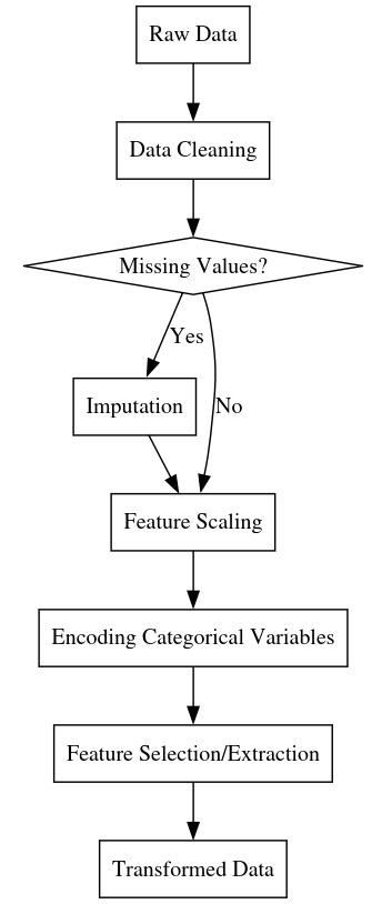
2.4.1 Data Preparation

The first and arguably most important step in any machine learning project is preparing the data. As we saw in Section 6.2.2, the quality and representativeness of the training data is essential for learning meaningful patterns that generalize well to new examples. No amount of algorithmic sophistication can make up for fundamentally flawed or insufficient data.

Key aspects of data preparation include:

• Data cleaning: Identifying and correcting errors, inconsistencies, and missing values in the raw data. This can involve steps like removing duplicate records, standardizing formats, and imputing missing values based on statistical patterns.

• Feature engineering: Transforming the raw input data into a representation that is more amenable to learning. This can involve steps like normalizing numeric features, encoding categorical variables, extracting domain-specific features, and reducing dimensionality.

• Data augmentation: Increasing the size and diversity of the training set by generating new examples through transformations of the existing data. This is especially common in domains like computer vision, where techniques like random cropping, flipping, and color jittering can help improve the robustness of the learned models.

• Data splitting: Dividing the data into separate sets for training, validation, and testing. The training set is used to fit the model parameters, the validation set is used to tune hyperparameters and detect overfitting, and the test set is used to evaluate the final performance of the model on unseen data.

The specifics of data preparation will vary depending on the domain and the characteristics of the data, but the general principles of ensuring data quality, representativeness, and suitability for learning are universal. It’s often said that data preparation is 80% of the work in machine learning, and while this may be an exaggeration, it underscores the critical importance of getting the data right.

To make this more concrete, let’s consider an example of data preparation in the context of a real-world problem. Suppose we’re working on a machine learning system to predict housing prices based on features like square footage, number of bedrooms, location, etc. Our raw data might look something like this:

Address,Sq.Ft.,Beds,Baths,Price
123 Main St,2000,3,2.5,$500,000
456 Oak Ave,1500,2,1,"$350,000"
789 Elm Rd,1800,3,2,425000

To prepare this data for learning, we might perform the following steps:

• Standardize the ‘Price’ column to remove the “$” and “,” characters and convert to a numeric type.

• Impute missing values in the ‘Beds’ and ‘Baths’ columns (if any) with the median or most frequent value.

• Normalize the ‘Sq.Ft.’ column by subtracting the mean and dividing by the standard deviation.

• One-hot encode the ‘Address’ column into separate binary features for each unique location.

• Split the data into training, validation, and test sets in a stratified fashion to ensure representative price distributions in each split.

The end result might look something like this:

Sq.Ft._Norm,Beds,Baths,123_Main_St,456_Oak_Ave,789_Elm_Rd,...,Price
,3,2.5,1,0,0,...,500000
-0.58,2,1,0,1,0,...,350000
,3,2,0,0,1,...,425000
...

Of course, this is just a toy example, and in practice the data preparation process can be much more involved. The key point is that investing time and effort into carefully preparing the data is essential for building successful learning systems.

2.4.2 Model Selection and Training

Once the data is prepared, the next step is to select an appropriate model family and training procedure. As we saw in Section 6.3.3, this involves striking a balance between model complexity and generalization ability, often through a combination of cross-validation and regularization techniques.

Some key considerations in model selection include:

• Inductive biases: The assumptions and constraints that are built into the model architecture. For example, convolutional neural networks have an inductive bias towards translation invariance and local connectivity, which makes them well-suited for image recognition tasks.

• Parameter complexity: The number of learnable parameters in the model, which affects its capacity to fit complex patterns but also its potential to overfit to noise in the training data. Regularization techniques can help control parameter complexity.

• Computational complexity: The time and memory requirements for training and inference with the model. More complex models may require specialized hardware (like GPUs) and longer training times, which can be a practical limitation.

• Interpretability: The extent to which the learned model can be inspected and understood by humans. In some domains (like healthcare or finance), interpretability may be a key requirement for building trust and ensuring regulatory compliance.

The choice of model family will depend on the nature of the problem and the characteristics of the data. For structured data with clear feature semantics, “shallow” models like linear regression, decision trees, or support vector machines may be appropriate. For unstructured data like images, audio, or text, “deep” models like convolutional or recurrent neural networks are often used.

Once a model family is selected, the next step is to train the model on the prepared data. This typically involves the following steps:

• Instantiate the model with initial parameter values (e.g. random weights for a neural network).

• Define a loss function that measures the discrepancy between the model’s predictions and the true labels on the training set.

• Use an optimization algorithm (like stochastic gradient descent) to iteratively update the model parameters to minimize the loss function.

• Monitor the model’s performance on the validation set to detect overfitting and tune hyperparameters.

• Stop training when the validation performance plateaus or starts to degrade.

The specifics of the training process will vary depending on the chosen model family and optimization algorithm, but the general goal is to find the model parameters that minimize the empirical risk on the training data while still generalizing well to unseen examples.

To illustrate these ideas, let’s continue with our housing price prediction example. Suppose we’ve decided to use a regularized linear regression model of the form:

\[price = w_0 + w_1 * sqft + w_2 * beds + w_3 * baths + ...\]

where \(w_0, w_1, ...\) are the learned weights and sqft, beds, baths, ... are the input features.

We can train this model using gradient descent on the mean squared error loss function:

def mse_loss(y_true, y_pred):
    return np.mean((y_true - y_pred) ** 2)

def gradient_descent(X, y, w, lr=0.01, num_iters=100):
    for i in range(num_iters):
        y_pred = np.dot(X, w)
        error = y_pred - y
        gradient = 2 * np.dot(X.T, error) / len(y)
        w -= lr * gradient
    return w

# Add a bias term to the feature matrix
X = np.c_[np.ones(len(X)), X]  

# Initialize weights to zero
w = np.zeros(X.shape[1])

# Train the model
w = gradient_descent(X, y, w)

We can also add L2 regularization to the loss function to prevent overfitting:

def mse_loss_regularized(y_true, y_pred, w, alpha=0.01):
    return mse_loss(y_true, y_pred) + alpha * np.sum(w**2)

def gradient_descent_regularized(X, y, w, lr=0.01, alpha=0.01, num_iters=100):
    for i in range(num_iters):
        y_pred = np.dot(X, w)
        error = y_pred - y
        gradient = 2 * np.dot(X.T, error) / len(y) + 2 * alpha * w
        w -= lr * gradient
    return w

# Train the regularized model
w = gradient_descent_regularized(X, y, w)

The alpha parameter controls the strength of the regularization - larger values will constrain the weights more strongly, while smaller values will allow the model to fit the training data more closely.

By tuning the learning rate lr, regularization strength alpha, and number of iterations num_iters, we can find the model that achieves the best balance between fitting the training data and generalizing to new examples.

Of course, linear regression is just one possible model choice for this problem. We could also experiment with more complex models like decision trees, random forests, or neural networks, each of which would have its own set of hyperparameters to tune. The key is to use a combination of domain knowledge, empirical validation, and iterative refinement to find the model that best suits the problem at hand.

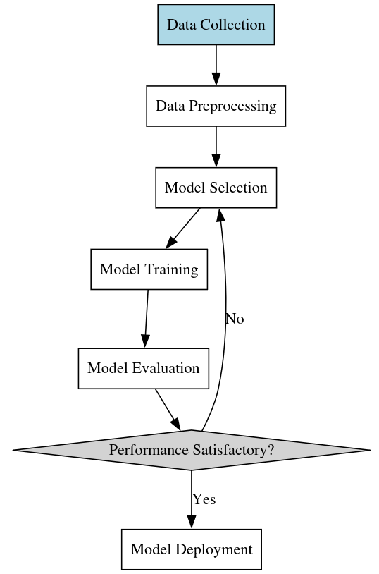
2.4.3 Model Evaluation and Deployment

Once we’ve trained a model that performs well on the validation set, the final step is to evaluate its performance on the held-out test set. This gives us an unbiased estimate of how well the model is likely to generalize to real-world data.

Common evaluation metrics for classification problems include:

• Accuracy: The fraction of examples that are correctly classified.
• Precision: The fraction of positive predictions that are actually positive.
• Recall: The fraction of actual positives that are predicted positive.
• F1 Score: The harmonic mean of precision and recall.
• ROC AUC: The area under the receiver operating characteristic curve, which measures the tradeoff between true positive rate and false positive rate.

For regression problems, common metrics include:

• Mean squared error (MSE): The average squared difference between the predicted and actual values.
• Mean absolute error (MAE): The average absolute difference between the predicted and actual values.
• R-squared (R²): The proportion of variance in the target variable that is predictable from the input features.

It’s important to choose an evaluation metric that aligns with the business goals of the problem. For example, in a fraud detection system, we might care more about recall (catching as many fraudulent transactions as possible) than precision (avoiding false alarms), while in a medical diagnosis system, we might care more about precision (avoiding false positives that could lead to unnecessary treatments).

If the model’s performance on the test set is satisfactory, we can proceed to deploy it in a production environment. This involves integrating the trained model into a larger software system that can apply it to new input data and surface the predictions to end users.

Some key considerations in model deployment include:

• Scalability: Can the model handle the volume and velocity of data in the production environment? This may require techniques like batch processing, streaming, or distributed computation.

• Latency: How quickly does the model need to generate predictions in order to meet business requirements? This may require optimizations like model compression, quantization, or hardware acceleration.

• Monitoring: How will the model’s performance be monitored and maintained over time? This may involve tracking key metrics, detecting data drift, and periodically retraining the model on fresh data.

• Security: How will the model and its predictions be protected from abuse or unauthorized access? This may involve techniques like input validation, output filtering, or access controls.

Deploying and maintaining machine learning models in production is a complex topic that requires close collaboration between data scientists, software engineers, and domain experts. It’s an active area of research and development, with new tools and best practices emerging regularly.

To bring everything together, let’s return one last time to our housing price prediction example. After training and validating our regularized linear regression model, we can evaluate its performance on the test set:

from sklearn.metrics import mean_squared_error, mean_absolute_error, r2_score

# Generate predictions on the test set
y_pred = np.dot(X_test, w)

# Calculate evaluation metrics
mse = mean_squared_error(y_test, y_pred)
mae = mean_absolute_error(y_test, y_pred)
r2 = r2_score(y_test, y_pred)

print(f"Test MSE: {mse:.2f}")
print(f"Test MAE: {mae:.2f}")
print(f"Test R^2: {r2:.2f}")

If we’re satisfied with the model’s performance, we can deploy it as part of a larger housing price estimation service. This might involve:

• Wrapping the trained model in a web service API that can accept new housing features and return price predictions.

• Integrating the API with a user-facing application that allows homeowners or real estate agents to input property information and receive estimates.

• Setting up a data pipeline to continuously collect new housing data and periodically retrain the model to capture changing market conditions.

• Defining monitoring dashboards and alerts to track the model’s performance over time and detect any anomalies or degradations.

• Establishing governance policies and processes for managing the lifecycle of the model, from development to retirement.

Again, this is a simplified example, but it illustrates the end-to-end process of building a machine learning system, from data preparation to model development to deployment and maintenance.

2.5 The Ethics and Governance of Machine Learning

As machine learning systems become more prevalent and powerful, it’s crucial that we grapple with the ethical implications of their development and deployment. In this final section, we’ll explore some key ethical considerations and governance principles for responsible machine learning.

2.5.1 Fairness and Bias

One of the most pressing ethical challenges in machine learning is ensuring that models are fair and unbiased. If the training data reflects historical biases or discrimination, the resulting model may perpetuate or even amplify those biases in its predictions.

For example, consider a hiring model that is trained on past hiring decisions to predict the likelihood of a candidate being successful in a job. If the training data comes from a company with a history of discriminatory hiring practices, the model may learn to penalize candidates from underrepresented groups, even if those factors are not actually predictive of job performance.

Detecting and mitigating bias in machine learning systems is an active area of research, with techniques like:

• Demographically balancing datasets to ensure equal representation of different groups

• Adversarial debiasing to remove sensitive information from model representations

• Regularization techniques to penalize models that exhibit disparate impact

• Post-processing methods to adjust model outputs to satisfy fairness constraints

However, these techniques are not perfect, and there is often a tradeoff between fairness and accuracy. Moreover, fairness is not a purely technical issue, but a sociotechnical one that requires ongoing collaboration between machine learning practitioners, domain experts, policymakers, and affected communities.

2.5.2 Transparency and Accountability

Another key ethical principle for machine learning is transparency and accountability. As models become more complex and consequential, it becomes harder for humans to understand how they arrive at their predictions and to trace the provenance of their training data and design choices.

This opacity can make it difficult to audit models for bias, safety, or compliance with regulations. It can also make it harder to challenge or appeal decisions made by machine learning systems, leading to a loss of human agency and recourse.

Some techniques for promoting transparency and accountability in machine learning include:

• Model interpretability methods that provide human-understandable explanations of model predictions

• Provenance tracking to document the lineage of data, code, and models used in a system

• Audit trails and version control to enable reproducibility and historical analysis

• Participatory design processes that involve affected stakeholders in the development and governance of models

However, like fairness, transparency is not purely a technical problem. It also requires institutional structures and processes for oversight, redress, and accountability. This might involve things like:

• Designating responsible individuals or teams for the ethical development and deployment of machine learning systems

• Establishing review boards or oversight committees to assess the social impact and governance of models

• Creating channels for affected individuals and communities to provide input and feedback on the use of machine learning in their lives

• Developing legal and regulatory frameworks to enforce transparency and accountability standards

2.5.3 Safety and Robustness

As machine learning systems are deployed in increasingly high-stakes domains, from healthcare to transportation to criminal justice, ensuring their safety and robustness becomes paramount. Models that are brittle, unreliable, or easily fooled can lead to serious harms if they are not carefully designed and tested.

Some key challenges in machine learning safety and robustness include:

• Distributional shift, where models trained on one data distribution may fail unexpectedly when applied to a different distribution

• Adversarial attacks, where malicious actors can craft inputs that fool models into making egregious errors

• Reward hacking, where optimizing for the wrong objective function can lead models to behave in unintended and harmful ways

• Safe exploration, where models need to learn about their environment without taking catastrophic actions

Techniques for improving the safety and robustness of machine learning systems include:

• Anomaly and out-of-distribution detection to flag inputs that are far from the training data

• Adversarial training and robustness regularization to make models more resilient to perturbations

• Constrained optimization and safe reinforcement learning to respect safety boundaries during learning

• Formal verification and testing to provide guarantees about model behavior under different conditions

However, building truly safe and robust machine learning systems requires more than just technical solutions. It also requires:

• Rigorous safety culture and practices throughout the development and deployment lifecycle

• Close collaboration between machine learning practitioners, domain experts, and safety professionals

• Proactive engagement with policymakers and the public to align the development of machine learning with societal values and expectations

• Ongoing monitoring and adjustment of deployed systems to catch and correct errors and unintended consequences

2.5.4 Ethical Principles and Governance Frameworks

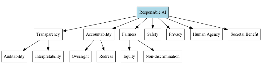
To navigate the complex ethical landscape of machine learning, we need clear principles and governance frameworks to guide responsible development and deployment. Some key principles that have been proposed include:

• Transparency: Machine learning systems should be auditable and understandable by humans.

• Accountability: There should be clear mechanisms for oversight, redress, and enforcement.

• Fairness: Machine learning should treat all individuals equitably and avoid discriminatory impacts.

• Safety: Machine learning systems should be reliable, robust, and safe throughout their lifecycle.

• Privacy: The collection and use of data for machine learning should respect individual privacy rights and provide appropriate protections.

• Human agency: Machine learning systems should respect human autonomy and dignity, and provide meaningful opportunities for human input and control.

• Societal benefit: The development and deployment of machine learning should be guided by considerations of social good and collective wellbeing.

Translating these high-level principles into practical governance frameworks is an ongoing challenge, but some key elements include:

• Ethical codes of conduct and professional standards for machine learning practitioners

• Impact assessment and risk management processes to identify and mitigate potential harms

• Stakeholder engagement and participatory design to ensure affected communities have a voice

• Regulatory sandboxes and policy experiments to test new governance approaches

• International standards and coordination to address the global nature of machine learning development

Ultimately, the goal of machine learning governance should be to ensure that the technology is developed and deployed in a way that aligns with human values and enhances, rather than undermines, human flourishing. This is a complex and ongoing process that will require sustained collaboration across disciplines, sectors, and geographies.

2.6 Conclusion

In this chapter, we’ve embarked on a comprehensive exploration of the foundations of machine learning, from its historical roots to its modern techniques to its future challenges. We’ve seen how the field has evolved from rule-based expert systems to data-driven statistical learning, powered by the explosion of big data and computing power. We’ve examined the fundamental components of machine learning systems - the data they learn from, the patterns they aim to extract, and the algorithms that power the learning process. We’ve discussed key concepts like inductive bias, generalization, overfitting, and regularization, and how they relate to the art of building effective models. We’ve walked through the practical steps of constructing a machine learning pipeline, from data preparation to model selection to deployment and monitoring. And we’ve grappled with some of the ethical challenges and governance principles that arise when building systems that can have significant impact on people’s lives.

The field of machine learning is still rapidly evolving, with new breakthroughs and challenges emerging every year. As we look to the future, some of the key frontiers and open questions include:

• Continual and lifelong learning: How can we build models that can learn continuously and adapt to new tasks and domains over time, without forgetting what they’ve learned before?

• Causality and interpretability: How can we move beyond purely associational patterns to uncover causal relationships and build models that are more interpretable and explainable to humans?

• Robustness and safety: How can we guarantee that machine learning systems will behave safely and reliably, even in the face of distributional shift, adversarial attacks, or unexpected situations?

• Human-AI collaboration: How can we design machine learning systems that augment and empower human intelligence, rather than replacing or undermining it?

• Ethical alignment: How can we ensure that the development and deployment of machine learning aligns with human values and promotes beneficial outcomes for society as a whole?

Advancing machine learning requires collaboration across disciplines—from computer science and statistics to psychology, social science, philosophy, and ethics. It also demands engagement with policymakers, industry leaders, and the public to ensure responsible and inclusive development. The goal is to build systems that learn from experience to make decisions that benefit humanity, whether in healthcare, scientific discovery, or improving daily life.

However, realizing this potential goes beyond technical progress; it requires addressing fairness, accountability, transparency, and safety while navigating ethical and governance challenges. Machine learning practitioners must not only push technological boundaries but also consider the broader impact of their work. By embracing diverse perspectives and collaborating beyond our field, we shape the future of AI. Staying curious, critical, and committed to responsible development will ensure machine learning serves society for generations to come.